- Keep two windows open, one with these instructions and the other with the flux study web pages.
- Go back and forth between them.
- Use the scroll bar to move the instructions.
- Look for the blue highlights for guidance.
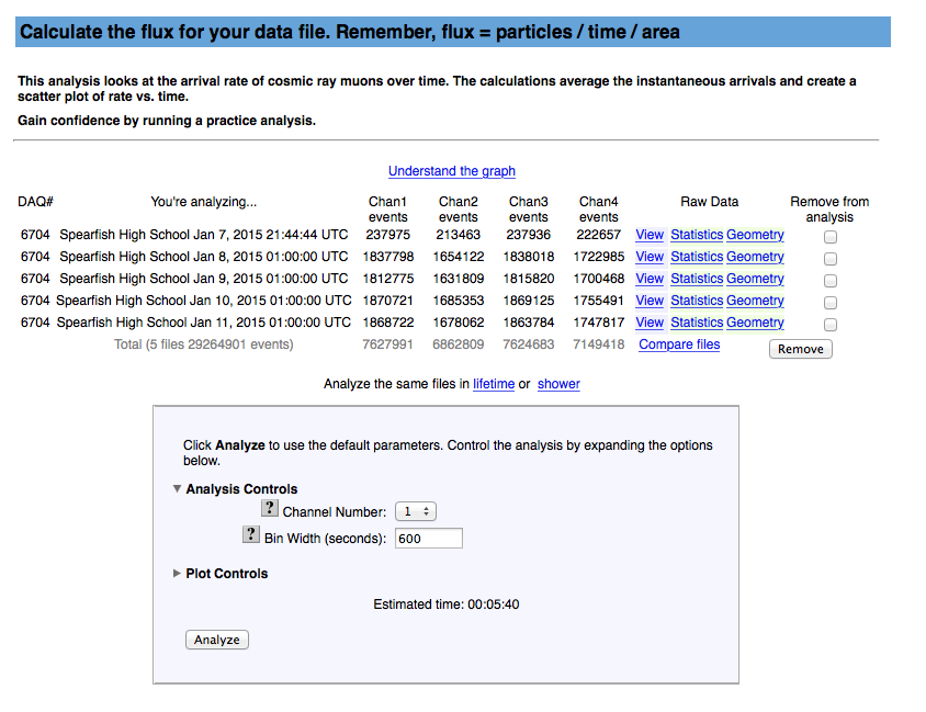
We shall create a plot with data from detector 6704 at Spearfish High School dated 01/07/15 through 01/11/15 (MM/DD/YYYY).
|
| |
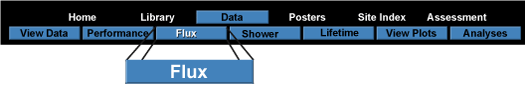
| Step 1: | Click on the Data button in the main menu. |
 |
| |
| Step 2: | Click on the Flux button in the submenu. |
 |
| |
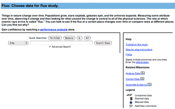
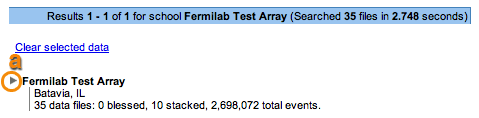
| Step 3.1: | Look at the search page. On the right, we have links to a tutorial, step-by-step instructions, FAQs and related milestones. The legend shows icons for information about each data file. |
 |
| |
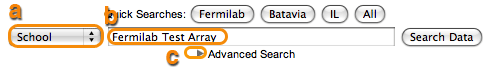
| Step 3.2: | Search for data files from Spearfish High School for January 2015.
a) Select School in the pulldown list.
b) Enter Spearfish High School in the search field.
c) Click on the little arrow next to "Advanced Search." |
 |
|
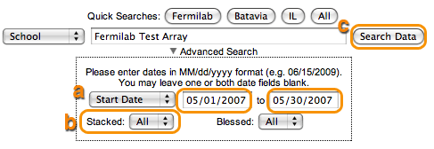
| Step 3.3: |
a) Select Start Date in the pulldown list. Enter "1/1/2015" in the first date field and "1/31/15" in the second date field. One can also use the calendar to select these dates.
b) Select Yes in the pull-down list for Stacked.
c) Click Search Data.
Note: 'Blessed Default' refers to data files that have been blessed. To retreive all data files (blessed and unblessed), choose 'Blessed All'. |
 |
|
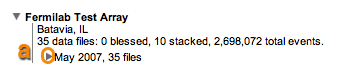
| Step 3.4: | a) Click on the little arrow next to "Spearfish High School" to see the data files.
|
 |
|
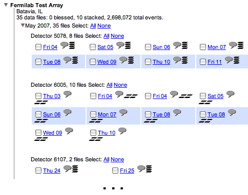
| Step 3.5: | a) Click on the little arrow next to "January 2015" to see the data files for that month.
|
 |
|
| Step 3.6: | All the data files uploaded for January 2015 are displayed. Notice there are files from two detectors.
See the data by clicking on the magnifying glass icon  next to the date and additional information by clicking on the comments bubble next to the date and additional information by clicking on the comments bubble  . . |
 |
| |
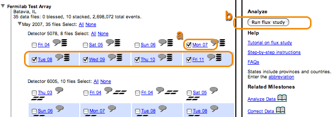
| Step 4: | We shall select data from detector 6704.
a) To select data for analysis, select the checkboxes next to "Wed 07," "Thu 08," "Fri 09." "Sat 10," and "Sun 11."
b) Click Run flux study. |
 |
| |
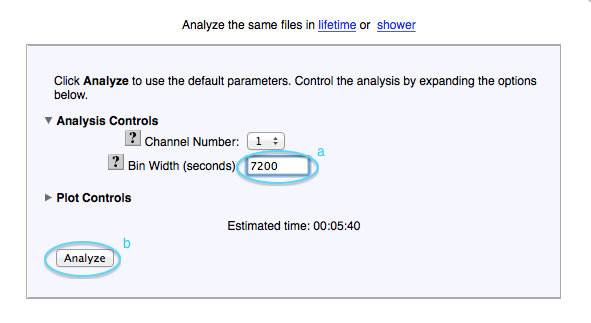
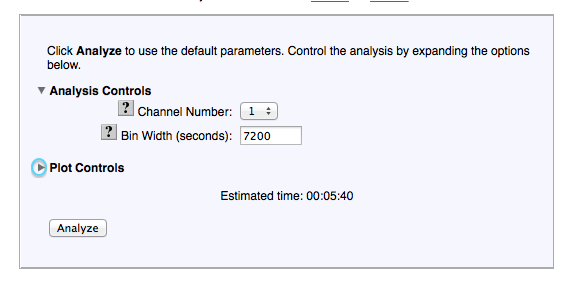
| Step 5: | We shall analyze events in channel 1. Flux will count the number of times an event was recorded by the DAQ in which channel 1 was present. |
 |
| | a.) Change the Bin Width to 7200.
b.) Click Analyze. |
 |
| |
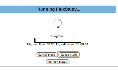
| Step 5.1: | If the analysis takes very little time to run, the plot may show up quickly. More often, though, one gets a progress bar displaying how the analysis is doing.
One can click on Queue study to allow the analysis to continue in the background. |
 |
| |
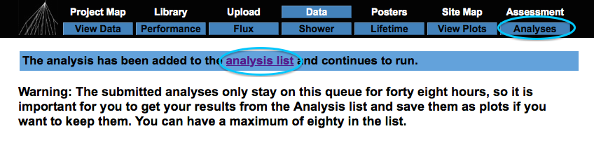
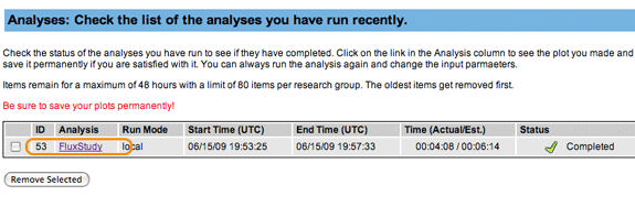
| Step 5.2: | One can click on Analyses on the navigation bar or analysis list in the text to see the job's progress. |
 |
| |
| Step 5.3: | When the job is done, an entry will appear in the Analysis List like this. Click on the link and see the plot. |
 |
| |
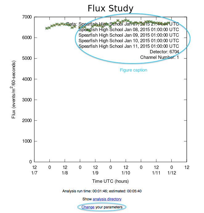
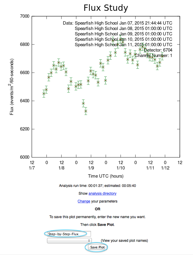
| Step 6: | Here's the graph of the flux - a histogram showing the number of events/m2/60 seconds ( = number⁄60m2·s) from January 7, 2015, through January 11, 2015. The Figure caption for the data files covers only some of the points. So, one can change the maximum y value in the plot or change the Figure caption (both found under Plot Controls).
Click Change your parameters to alter the plot. |
 |
| |
| Step 7: | Click on the small arrow to view the Plot Controls. |
 |
| |
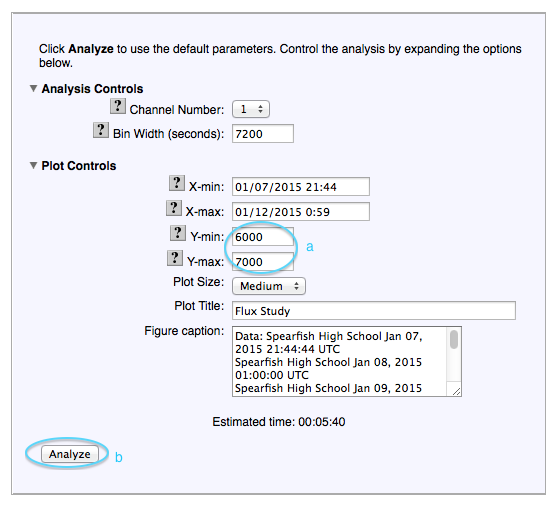
| Step 8: | Try varying some of the plot controls.
a) Enter 6000 as Y-min and 7000 as Y-max.
b) Click Analyze. |
 |
| |
| Step 8.1: | When the progress bar appears, one can queue the study and then go to it from the analysis list. As described above, click on the study name when it is completed to see the plot. |
| |
| Step 9: | Here is the new plot. The legend for the data files includes the data points. Save it.
Enter a name for the plot and click Save Plot. Choose a different name each time through the tutorial.
This plot can be accessed for the poster.
|
 |
| |
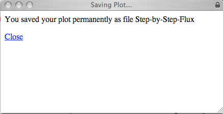
| Step 10: | Note the successfully saved plot. Click Close.
One can create more plots for other channels or go back to choosing a new data set by clicking Flux. At any time, click View Plots to see the plots. One can also run any study again from the saved plot.
|
 |