- Keep two windows open, one with these instructions and the other with the TOF study web pages.
- Go back and forth between them.
- Use the scroll bar to move the instructions.
- Look for the blue highlights for guidance.
We shall create a plot with data collected at Fermilab with DAQ #6203 from November 2015 to January 2016.
|
| |
| Step 1: | Click on the Data button in the main menu. |
 |
| |
| Step 2: | Click on the Shower button in the submenu. |
 |
| |
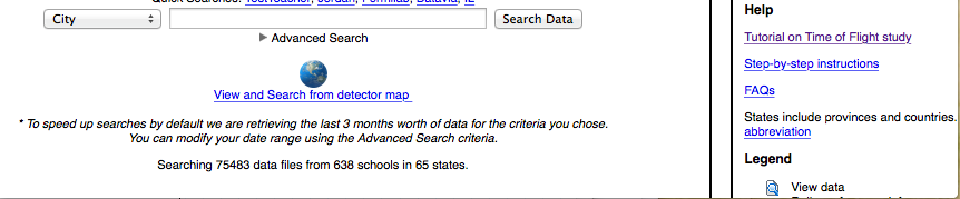
| Step 3.1: | Look at the search page. On the right, there are links to a tutorial, step-by-step instructions, and FAQs. The legend shows icons for information about each data file.
NOTE: TOF works with one file at a time. So, we use Advanced Search to select one file. |
 |
| |
| Step 3.2: |
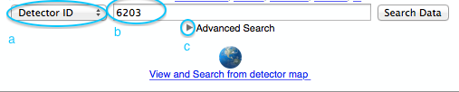
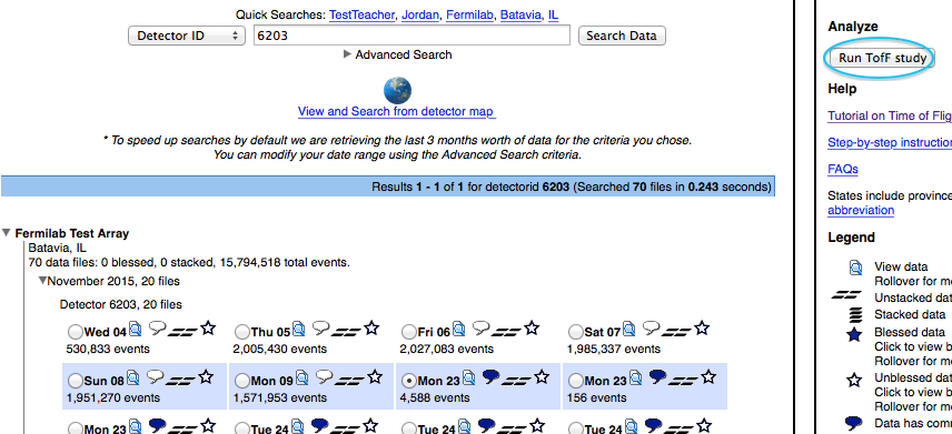
Find all data for DAQ #6203 from Nov. 1, 2015 through Jan. 31, 2016.
a) Select Detector ID in the pulldown list.
b) Enter 6203 in the search field.
c) Click on the little arrow next to "Advanced Search." |
 |
|
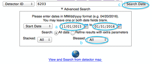
| Step 3.3: | a) Select Start Date in the pulldown list for dates and enter "11/01/2015" in the first date field and "01/31/2016" in the second date field. You can also use the calendar.
b) Select Blessed: All. This means all files, blessed or not. Default means blessed only.
c) Click Search Data |
 |
|
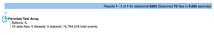
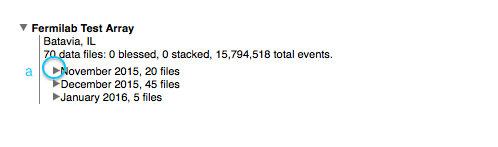
| Step 3.4: | a) Click on the little arrow next to "Fermilab Test Array" to see the data files.
|
 |
|
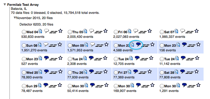
| Step 3.5: | a) Click on the little arrow next to "November 2015" to see the data files for that month.
|
 |
|
| Step 3.6: | One can view the data by clicking on the icon with the magnifying glass and additional information by clicking on the comments bubble. |
 |
| |
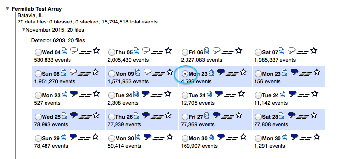
| Step 4: | Click the button next to the first Monday, 11/23/2015, data set.
|
 |
|
| Step 4.1: | Then click Run TOF study on the right.
|
 |
|
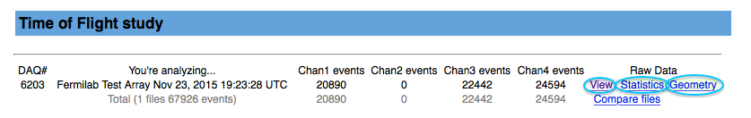
| Step 4.2: | Look at the display of the selected data file. You can view the raw data and check the statistics. Also, make sure the geometry file is there.
|
 |
| |
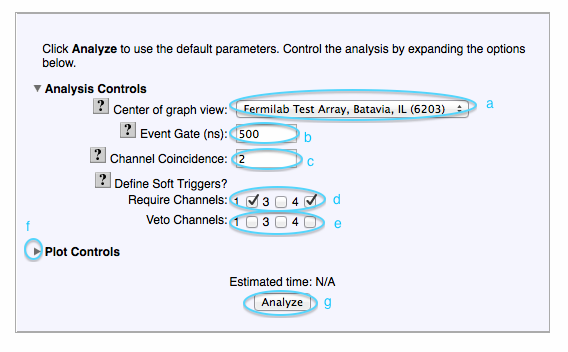
| Step 5: | To understand the input parameters, you can click on the question mark next to each. The first time through, keep all the defaults,
a) DAQ Name: Fermilab Test Array, Batavia, IL (6203).
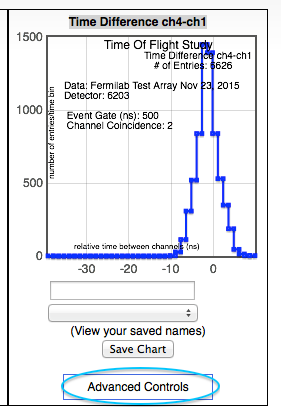
b) Event gate (ns): 500.
c) Channel Coincidence: 2.
d) Define Soft Triggers? Require Channels: None, in the case of the first example given in the TOF Tutorial. Software triggers are used in the later examples.
e) Define Soft Triggers? Veto Channels: None.
f) Plot Controls: As an option, you can modify labels on the plot.
g) Click Analyze. We will run the analysis on our local computer. This will take a while, so don't be alarmed if you do not get a plot right away. |
 |
| |
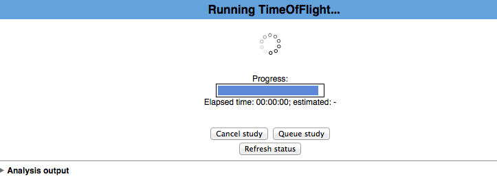
| Step 5.1: | If your analysis takes very little time to run, you may get your plot right away. More often, you get a progress bar displaying how the analysis is doing. You can click on Queue study to allow the analysis to go on in the background. You can also click on Analysis output to see the inner workings. This might
help you if you encounter an error in your analysis. |
 |
| |
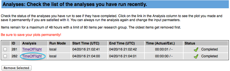
| Step 5.2: | You can now click on Analyses on the navigation bar to see the progress of you job. |
 |
| |
| Step 5.3: | When your job is done, you will see an entry on the Analysis List like this. You can click on the link and see the plot.
|
 |
| |
| Step 6: | On the Time Difference ch4-ch1 plot, click Advanced Controls. |
 |
| |
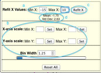
| Step 7.1: | Limit the interval of the x-axis where the fit is applied. This step can be used to eliminate tails or background.
a) Change the Min X to -15 and Max X to 10.
b) Keep the other settings (X-axis & Y-axis scale and Bin Width). Changing the bin width is not compatible with refitting the x-values.
c) Click Refit X.
d) Notice: Mean and standard deviation may change for the new internal.
|
 |
| |
| Step 7.2: | Result of Refit X: |
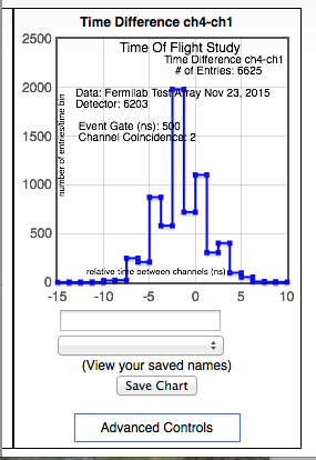 |
| Notice: | Data seems to jump up and down. Because the DAQ measures in 1.25ns steps, there can be odd correlations between the two counters, leading to a ragged plot. |